library(gapminder) # provides gapminder dataset
library(tidyverse)
library(ggplot2)

library(plotly) # for interactive plots
library(gganimate) # for animated plots
library(knitr) # for kable tables
library(kableExtra) # for even prettier kable tables
library(tableone) # for baseline characteristics table2 Tables and Plots
2.1 gapminder dataset
Country-specific data from 1952 to 2007 with the following variables: country, continent, year, lifeExp, pop, and gdpPercap.
2.2 Tables
Base R table Function or Manual Data Manipulation
table(gapminder$continent)
  Africa Americas     Asia   Europe  Oceania
     624      300      396      360       24
gapminder %>%
dplyr::select(-c(country, year)) %>%
dplyr::group_by(continent) %>%
dplyr::summarize_all(mean)# A tibble: 5 × 4
continent lifeExp pop gdpPercap
<fct> <dbl> <dbl> <dbl>
1 Africa 48.9 9916003. 2194.
2 Americas 64.7 24504795. 7136.
3 Asia 60.1 77038722. 7902.
4 Europe 71.9 17169765. 14469.
5 Oceania 74.3 8874672. 18622.Kable tables
Bootstrap Theme
t(table(gapminder$continent)) %>%
  kableExtra::kbl() %>%
  kableExtra::kable_styling()
Africa Americas Asia Europe Oceania 624 300 396 360 24 Paper theme
t(table(gapminder$continent)) %>%
  kableExtra::kbl() %>%
  kableExtra::kable_paper(
    "hover", full_width = F
  )
Africa Americas Asia Europe Oceania 624 300 396 360 24 Classic theme
t(table(gapminder$continent)) %>%
  kableExtra::kbl() %>%
  kableExtra::kable_classic(
    full_width = F,
    position = 'left'
  )
Africa Americas Asia Europe Oceania 624 300 396 360 24
Table One
Basic Baseline Characteristics
tab = tableone::CreateTableOne(
  data = gapminder,
  vars = c('continent','lifeExp','pop','gdpPercap')
)

tab
Overall n 1704 continent (%) Africa 624 (36.6) Americas 300 (17.6) Asia 396 (23.2) Europe 360 (21.1) Oceania 24 ( 1.4) lifeExp (mean (SD)) 59.47 (12.92) pop (mean (SD)) 29601212.32 (106157896.74) gdpPercap (mean (SD)) 7215.33 (9857.45)summary(tab)### Summary of continuous variables ### strata: Overall n miss p.miss mean sd median p25 p75 min max skew kurt lifeExp 1704 0 0 6e+01 1e+01 6e+01 5e+01 7e+01 24 8e+01 -0.3 -1 pop 1704 0 0 3e+07 1e+08 7e+06 3e+06 2e+07 60011 1e+09 8.3 78 gdpPercap 1704 0 0 7e+03 1e+04 4e+03 1e+03 9e+03 241 1e+05 3.9 28 ======================================================================================= ### Summary of categorical variables ### strata: Overall var n miss p.miss level freq percent cum.percent continent 1704 0 0.0 Africa 624 36.6 36.6 Americas 300 17.6 54.2 Asia 396 23.2 77.5 Europe 360 21.1 98.6 Oceania 24 1.4 100.0Stratify Table
tab2 = tableone::CreateTableOne(
  data = gapminder,
  vars = c('lifeExp','pop','gdpPercap'),
  strata = 'continent'
)
tab2
Stratified by continent Africa Americas n 624 300 lifeExp (mean (SD)) 48.87 (9.15) 64.66 (9.35) pop (mean (SD)) 9916003.14 (15490923.32) 24504795.00 (50979430.20) gdpPercap (mean (SD)) 2193.75 (2827.93) 7136.11 (6396.76) Stratified by continent Asia Europe n 396 360 lifeExp (mean (SD)) 60.06 (11.86) 71.90 (5.43) pop (mean (SD)) 77038721.97 (206885204.62) 17169764.73 (20519437.65) gdpPercap (mean (SD)) 7902.15 (14045.37) 14469.48 (9355.21) Stratified by continent Oceania p test n 24 lifeExp (mean (SD)) 74.33 (3.80) <0.001 pop (mean (SD)) 8874672.33 (6506342.47) <0.001 gdpPercap (mean (SD)) 18621.61 (6358.98) <0.001Save Table to CSV
tab2_mat = print(tab2, quote = FALSE, nospaces = TRUE, printToggle = FALSE)
write.csv(tab2_mat, file = "myTableOne.csv")
Copy Table into LaTeX document (need to run in Console)
knitr::kable(tab2_mat, format = 'latex')
Combining Kable and TableOne
tab2_mat %>%
  kableExtra::kbl() %>%
  kableExtra::kable_paper(
    "hover"
)| Africa | Americas | Asia | Europe | Oceania | p | test | |
|---|---|---|---|---|---|---|---|
| n | 624 | 300 | 396 | 360 | 24 | ||
| lifeExp (mean (SD)) | 48.87 (9.15) | 64.66 (9.35) | 60.06 (11.86) | 71.90 (5.43) | 74.33 (3.80) | <0.001 | |
| pop (mean (SD)) | 9916003.14 (15490923.32) | 24504795.00 (50979430.20) | 77038721.97 (206885204.62) | 17169764.73 (20519437.65) | 8874672.33 (6506342.47) | <0.001 | |
| gdpPercap (mean (SD)) | 2193.75 (2827.93) | 7136.11 (6396.76) | 7902.15 (14045.37) | 14469.48 (9355.21) | 18621.61 (6358.98) | <0.001 |
2.3 Figures
This example builds upon one on the gganimate website
ggplot: we can’t tell which year is which!
plot1 = ggplot2::ggplot(
  gapminder,
  aes(
    x = gdpPercap,
    y = lifeExp,
    size = pop,
    color = country,
    text = paste('Year:',year)
  )
) +
  geom_point(alpha = 0.7, show.legend = FALSE) +
  scale_colour_manual(values = country_colors) +
  scale_size(range = c(2, 12)) +
  scale_x_log10() +
  facet_wrap(~continent) +
  labs(
    x = 'GDP per capita',
    y = 'life expectancy'
  )

plot1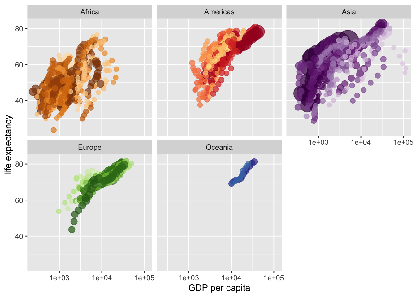
plotly: we can hover to identify points for each country/year
Note: Only variables in aes() show up in the tooltip by default. A trick I used here is to add a text aesthetic to add the year to the tooltip.
plotly::ggplotly(plot1)gganimate: visually see data move over the years
Basics of gganimate:
transition_time(),transition_states():how the data should be spread out across timeenter_*(),exit_*(): how new data should appear and old data should disappear (e.g. fade in, shrink out)
Note: you need to install gifski and png packages before running the code below.
plot1 +
  transition_time(year) +
  labs(
    title = 'Year: {frame_time}'
  )